

Dates and Events:
|
OSADL Articles:
2023-11-12 12:00
Open Source License Obligations Checklists even better nowImport the checklists to other tools, create context diffs and merged lists
2022-07-11 12:00
Call for participation in phase #4 of Open Source OPC UA open62541 support projectLetter of Intent fulfills wish list from recent survey
2022-01-13 12:00
Phase #3 of OSADL project on OPC UA PubSub over TSN successfully completedAnother important milestone on the way to interoperable Open Source real-time Ethernet has been reached
2021-02-09 12:00
Open Source OPC UA PubSub over TSN project phase #3 launchedLetter of Intent with call for participation is now available |
 embedded world Conference 2025
 embedded world Conference 2025
HOWTO: Create a pseudo 3D long-term latency graphic derived from a large number of consecutive latency plots
Create a set of test data
In a first step, we need to create some test data that must be formatted in the same way as the actual plot data:
<Number (µs)> <space> <frequency core #0> <tabulator> <frequency core #1> <tabulator> <frequency core #N>
To do so, we run the following script:
#!/bin/bash

echo=`which echo`

for i in `seq 1 180`
do
  core0=`expr 90000000 - $i \* 360000`
  core1=`expr 80000000 - $i \* 360000`
  core2=`expr 70000000 - $i \* 360000`
  core3=`expr 80000000 - $i \* 360000`
  rm -f latency-$i
  for j in `seq 0 399`
  do
    $echo -e `printf %06d $j` $core0\\t$core1\\t$core2\\t$core3 >>latency-`printf %03d $i`
    core0=`expr $core0 - 500000`; if test $core0 -lt 0; then core0=0; fi;
    core1=`expr $core1 - 500000`; if test $core1 -lt 0; then core1=0; fi;
    core2=`expr $core2 - 500000`; if test $core2 -lt 0; then core2=0; fi;
    core3=`expr $core3 - 500000`; if test $core3 -lt 0; then core3=0; fi;
  done
done

sed -i "s/200 0/200 1/" latency-090
which will create a total of 180 simulated data files named latency-001 to latency-180 in the same format as if they had been obtained form cyclictest running in histogram mode on a 4-core processor. An artificial single outlier with a latency of 200 µs occurring at latency plot #90 is inserted.
Create the pseudo 3D graphic with R
This R script will read the data, select the highest value per line, transform them to a 3D matrix and call the persp() routine to generate the graphic.
read.matrix <-
function(file, header = FALSE, sep = "", skip = 0)
{
  row.lens <- count.fields(file, sep = sep, skip = skip)
  if(any(row.lens != row.lens[1]))
    stop("number of columns is not constant")
  if(header) {
    nrows <- length(row.lens) - 1
    ncols <- row.lens[2]
    col.names <- scan(file, what = "", sep = sep, nlines = 1, quiet = TRUE, skip = skip)
    x <- scan(file, sep = sep, skip = skip + 1, quiet = TRUE)
  }
  else {
    nrows <- length(row.lens)
    ncols <- row.lens[1]
    x <- scan(file, sep = sep, skip = skip, quiet = TRUE)
    col.names <- NULL
  }
  x <- as.double(x)
  if(ncols > 1) {
    dim(x) <- c(ncols,nrows)
    x <- t(x)
    colnames(x) <- col.names
  }
  else if(ncols == 1)
    x <- as.vector(x)
  else
    stop("wrong number of columns")
  return(x)
}

read.latencyplots <-
function(dir = ".")
{
  i <- 1
  files <- dir(".")
  files <- sort(files, decreasing = TRUE)
  r = read.delim(files[1], sep = "\n")
  rows = dim(r)[1] + 1
  z <- matrix(nrow = rows, ncol = length(files))
  for (file in files) {
    m <- read.matrix(file=file)
    m[,1] <- 0
    m <- apply(m, 1, max, na.rm = TRUE)
    z[,i] <- m
    i <- i + 1
  }
  return(z)
}

data = read.latencyplots(dir = ".")
data <- data + 0.1
data <- log10(data)
z <- data

x <- 1:nrow(z)
x <- c(min(x) - 1e-10, x, max(x) + 1e-10)

y <- 1:ncol(z)
y <- c(min(y) - 1e-10, y, max(y) + 1e-10)

z0 <- min(z)
z <- rbind(z0, cbind(z0, z, z0), z0)
fill <- matrix("green3", nrow = nrow(z)-1, ncol = ncol(z)-1)
fill[ , i2 <- c(1,ncol(fill))] <- "gray"
fill[i1 <- c(1,nrow(fill)) , ] <- "gray"
par(bg = "slategray")
fillfunc <- colorRampPalette(c("green", "yellow", "red"), space = "Lab",  interpolate = "spline")
fcol <- fill ; fcol[] <- fillfunc(nrow(fcol))

pdf("../3Dplot.pdf", paper = "special", width = 11.69, height = 8.26)
par(fin = c(10.69, 7.26), mai = c(0.5, 0.5, 0.5, 0.5), ps = 12, pty = "m")
persp(x, y, z, theta = 30, phi = 25, col = fcol, scale = FALSE, expand = 10 * nrow(z) / 200, nticks = 10, ticktype = "detailed",
  ltheta = -70, shade = 0.4, border = NA, box = TRUE, axes = TRUE, xlab = "Latency (us)", r = sqrt(3),
  zlab = "Frequency (log10)", ylab = "Repetitions")
title(main = "3D plot", font.main = 4)
Run the scripts and display the result
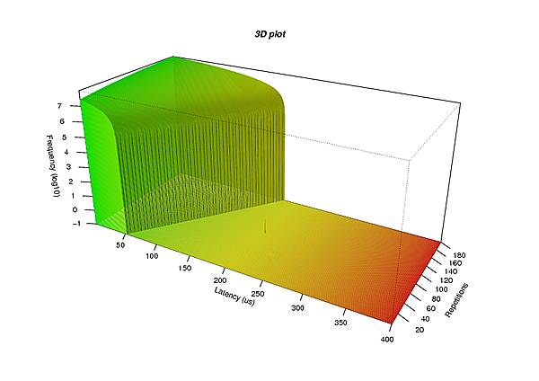
- Output of the R script (click on the image to show the PDF file)
To download and run the scripts type
cd /tmp
wget https://www.osadl.org/uploads/media/mkplotdata.bash
chmod +x mkplotdata.bash
wget https://www.osadl.org/uploads/media/mk3dplot.R
mkdir 3D
cd 3D
../mkplotdata.bash
R -f ../mk3dplot.R
cd ..
evince 3Dplot.pdf
and a graphic similar to the one at the right will be displayed. It may then further be processed with usual image converters to create bitmap files in a desired format.
Note that – due to the logarithmic vertical scale – the single outlier in the amount of 200 µs is distinguishable out of the many million recordings at latency plot #90.
Download the scripts
Bash script to create simulated plot data | 699 |
R script to generate the 3D graphic | 2.2 K |
Animated 3D
Finally, you may wish to create an animated sequence in order to allow for a better inspection of the whole of the results – particularly not to overlook single latency outliers. For this purpose, the R script is repeated with different view angles, and the resulting images are combined in an animated gif.

- Click on the image to show the animation
Optional video clips
If you really wanted, you may even produce short video clips from the animated GIF that have considerably shorter files sizes, but a less good resolution.
Video clip in AVI format | 851 K |
Video clip in Ogg-Vorbis format | 1.8 M |